Copy and Paste Multiple Items Using Office Clipboard

Copy and Paste Multiple Items by using the Office Clipboard

The Microsoft Office Clipboard allows you to copy multiple text and graphical items from Office documents or other programs and paste them into another Office document. For example, you can copy text from an e-mail message, data from a workbook or datasheet, and a graphic from a presentation and then paste them all into a Word document. By using the Office Clipboard, you can arrange the copied items the way that you want in the document.

Copy Multiple Items to the Office Clipboard

1. Open the file that you want to copy items from.
2. Select the first item that you want to copy.
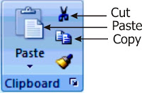
3. In these Office programs: Access, Excel, Outlook, PowerPoint, or Word; on the Home tab, in the Clipboard group, click Copy or press CTRL+C on the keyboard.
4. Continue copying items from the same or other files until you have collected all of the items that you want. The Office Clipboard can hold up to 24 items. If you copy a twenty-fifth item, the first item on the Office Clipboard is deleted.

If you open the Clipboard task pane in one Office program, the Clipboard task pane does not automatically appear when you switch to another Office program. However, you can continue to copy items from other programs. If the Show Status Near Taskbar When Copying option is selected, a message is displayed above the status area to indicate that an item has been added to the Office Clipboard.

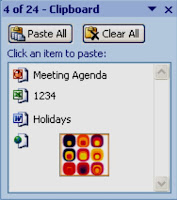
As items are added to the Office Clipboard, an entry is displayed in the Clipboard task pane. The newest entry is always added to the top. Each entry includes an icon representing the source Office program and a portion of copied text or a thumbnail of a copied graphic.

Collected items remain on the Office Clipboard until you exit all Office programs that are running on your computer or click Clear All in the Clipboard task pane. For more information, see Delete items from the Office Clipboard.

Paste Items

You can paste items from the Office Clipboard individually or all at the same time.

1. Click where you want the items to be pasted and do one of the following:
1. To paste items one at a time, in the Clipboard task pane, double-click each item that you want to paste.
2. To paste all the items that you copied, in the Clipboard task pane, click Paste All.
3. The Office Clipboard does not support the Paste Special command though it is available in Office programs.

Delete Items from the Office Clipboard

You can delete items from the Office Clipboard individually or all at the same time.

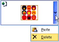
1. In the Clipboard task pane, do one of the following:
1. To clear one item, click the arrow next to the item that you want to delete, and then click Delete.
2. To clear all items, click Clear All.

Copying and Moving Data

The copy or Cut command can be used to duplicate or move highlighted data or formula. When you copy and paste, you are making a duplicate copy of the contents of one or more cells and placing the copy into another cell or range of cells, so you can copy entire cells or their contents.

On the other hand, when you cut and paste, you are removing the contents of one cell or a range from the original location and placing them into another cell or range. You can also copy or cut specific contents or attributes from the cells. For example, you can copy the resulting value of a formula without copying the formula itself, or you can copy only the formula.

When you copy a cell by dragging or by clicking Cut or Copy, and Paste icons on the Standard toolbar, Microsoft Excel copies the entire cell, including formulas and their resulting values, comments, and cell formats. If the selected copy area includes hidden cells, Microsoft Excel also copies the hidden cells. If the paste area contains hidden rows or columns, you might need to unhide the paste area to see all of the copied cells.

Move or Copy Entire Cells

1. Select the cells that you want to move or copy.
2. On the Home tab, in the Clipboard group, do one of the following:

1. To move cells, click Cut . Keyboard shortcut is to press CTRL+X.
2. To copy cells, click Copy . Keyboard shortcut is to press CTRL+C.
3. Select the upper-left cell of the paste area.

Important.

To move or copy a selection to a different worksheet or workbook, click the sheet tab or switch to another workbook, and then select the upper-left cell of the paste area.

4. On the Home tab, in the Clipboard group, click Paste . Keyboard shortcut is to press CTRL+V.

Important.

1. To choose specific options when you paste cells, you can click the drop down arrow below Paste, and then choose your options. For instance, you can click 'Paste Special', where you can select only values, values and formulas, values and formats, etc.
2. Excel replaces existing data in the paste area when you cut and paste cells to move them.
3. When you copy cells, cell references are automatically adjusted. When you move cells, however, cell references are not adjusted, and the contents of those cells and of any cells that point to them may be displayed as reference errors. In this case, you will need to adjust the references manually.

Move or Copy Entire Cells by Using the Mouse

1. Select the cells or range of cells you want to move or copy.
2. Do one of the following:
1. To move the cell(s), point to the border of the selection. When the pointer becomes a move pointer , drag the cell(s) to another location.
2. To copy the cell(s), hold down CTRL while you point to the border of the selection. When the pointer becomes a copy pointer , drag the cell(s) to another location.

Insert Moved or Copied Cells between Existing Cells

1. Select the cells or range of cells that contains the data you want to move or copy.
2. On the Home tab, in the Clipboard group, do one of the following:
1. To move the selection, click Cut.
2. To copy the selection, click Copy.
3. Right-click the upper-left cell of the paste area, and then click Insert Cut Cells or Insert Copied Cells on the shortcut menu.
4. In the Insert Paste dialog box, click the direction to which you want to shift the surrounding cells.

Important.

These steps are use to change the location of a given data. Using these features, you can move and copy data between worksheets, workbooks, or other Windows applications. They do not replace existing data on the worksheet. Copy cell values, cell formats, or formulas only.

You can copy specific contents or attributes from the cells without copying the entire contents. For example, you can copy the resulting values of a formula without copying the formula itself, or you can copy only the formula, format of other attributes of cell(s).

When you paste copied data, you can achieve any of the following:

• Convert any formulas in the cell to the calculated values without overwriting the existing formatting.
• Paste only the cell formatting, such as font color or fill color (and not the contents of the cells).
• Paste only the formulas (and not the calculated values).

1. Select the cell or range of cells that contains the values, cell formats, or formulas that you want to copy.
2. On the Home tab, in the Clipboard group, click Copy.
3. Select the paste area or the cell where you want to paste.
4. On the Home tab, in the Clipboard group, click the arrow below Paste, and then do one of the following:
1. To paste values only, click Paste Values.
2. To paste cell formats only, click Paste Special, and then click Formats under Paste.
3. To paste formulas only, click Formulas.
4. To transpose the content, click Paste Special, and under Operation, select Transpose and the click Ok.

Transposing cell contents is changing data in column to re-arrange them in a row or vice versa.

Important.

If the copied formulas contain relative cell references, Excel adjusts the references (and the relative parts of mixed cell references) in the duplicate formulas. If the copied formulas contain absolute cell references, the references in the duplicate formulas are not changed. If you don't get the results that you want, you can also change the references in the original formulas to either relative or absolute cell references and then recopy the cells.

Defining Microsoft Excel Named Reference

Defining MS Excel Named Reference

A cell reference refers to a cell or a range of cells on a worksheet and tells Microsoft Excel where to look for the values or data that you want to use in a formula. With cell references, you can use data that is contained in different parts of a worksheet in one formula, or you can use the value from one cell in several formulas. You can also refer to cells on other worksheets in the same workbook.

Although cell numbers are at the foundation of everything Excel does, it's much easier to remember names, such as Item Number and Quantity, than it is to remember cell numbers, such as A1:C100. Excel makes this easy.

A name is a meaningful shorthand or a label that makes it easier to understand the purpose of a cell reference or constant. For example, the number 210 and the text "Quarterly Earnings" constants but Quarterly Earning makes more meaning. You can use the labels on a table to refer to the cells within its columns and rows. Examples of labels are “unit Price”, “Quantity” and “Total.” Alternatively, you can create descriptive names to represent cells, ranges of cells, formulas, or constant values.

Creating Microsoft Excel Named Range

1. To name a cell or range, select the range of cell(s) you want define name for.
2. Type the desired name in the Name box and press ENTER key.

OR

1. Right-click the selected range, click Name a Range.
2. Type the desired name and click Ok.

Change Cell Reference to a Named Range

If you have defined a name to a cell reference after you have entered a cell reference in a formula, you would need to update the existing cell references to the defined names. Do one of the following:

1. Select the range of cells that contains formulas in which you want to replace cell references with defined names.
2. Select a single, empty cell to change the references to names in all formulas on the worksheet.
3. On the Formulas tab, in the Defined Names group, click the arrow next to Define Name, and then click Apply Names.
4. In the Apply names box, click one or more names, and then click Ok.

 

Highlighting and Selecting Range of Cells

A range of cells are cells that are grouped together by selection and are treated as a singe cell. Therefore any operation performed on a range affects all the cells in the range. Before you can carry out a command or select a toolbar option, you may be required to select the cells that you want the command to apply to. You can apply a selected command to:

1. A single cell.
2. A row or column.
3. A range of cells.
4. Non- adjacent range.
5. An entire worksheet.
6. An entire workbook.

Steps

1. Click on the starting cell (top-leftmost cell or bottom-rightmost cell of the range you want to select.
2. Click and hold down the left mouse button and drag to the ending cell.
3. Release the mouse button.

OR

1. Click on the starting cell, press and hold down the SHIFT key on the keyboard.
2. Press the appropriate ARROW key on the keyboard to extend the selection till you have highlighted the entire range. Note: holding CTRL + SHIFT keys and pressing appropriate ARROW key will highlight all cells in the range.

OR

1. To select large range of cells, click on the starting cell, press and hold down the SHIFT key on the keyboard.
2. Click the ending cell.
3. You can also select the first cell in the range, and then press F8 to extend the selection by using the ARROW keys. To stop extending the selection, press F8 again.
4. Click the first cell in the range, and then hold down SHIFT while you click the last cell in the range. You can scroll to make the last visible cell .

Steps to Select an Entire Column or Row

1. Click the column heading i.e. the column letter or the row number.
2. Drag across the row or column headings. Or select the first row or column; then hold down SHIFT key while you select the last row or column.

Important

If the row or column contains data, CTRL+SHIFT+ARROW key selects the row or column to the last used cell. Pressing CTRL+SHIFT+ARROW key a second time selects the entire row or column.

Steps to Select Non-Adjacent Cells

This means to select cells that are not close to each other e.g. B3 – B20, E5 – H5, D10 – D25;

1. Hold down the CTRL key on the keyboard and select the range you want.
2. Select the first cell, press SHIFT + F8 key on the keyboard while you select other cells. To stop the selection, press SHIFT + F8 key again.

To Select Entire Worksheet

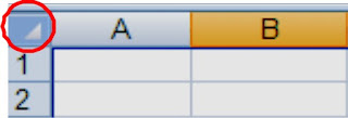
Click the 'Select All' button at the intersection of the column headers and row numbers tabs. You can also press CTRL+A on the keyboard.

Important

If the worksheet contains data, CTRL+A selects only the current region, but pressing CTRL+A a second time selects the entire worksheet.

Steps to Select Two or More Worksheets in a Workbook

1. For adjacent sheets, click the sheet tab of the first worksheet; Hold down Shift key on the keyboard and click the next Sheet tab.
2. For non-adjacent sheets, click the sheet tab of the first worksheet; Hold down CTRL on the keyboard and click the other Sheet tab(s).

How to Delete Data

Highlight the cell(s) whose data you wish to delete

Press delete key on the keyboard

Editing Data in a Cell

This has to do with correcting the content of a cell without having to re-type the entire the content.

1. Double click the cell whose content you want to edit.
2. Make your corrections.
3. Press Enter key or click outside the cell.

OR

1. Move the cell pointer to the cell containing the data or click on the cell.
2. Press F2 key on the keyboard.
3. Make your corrections.
4. Press Enter key or click outside the cell.

OR

1. Move the cell pointer to the cell containing the data or click on the cell.
2. Click on the formula bar.
3. Make your corrections on the formula bar.
4. Press Enter key or click outside the cell.

Deleting Unwanted Cells, Rows or Columns

1. Select a range you want to delete.
2. Click the Home menu.
3. Click the drop-down button under Cells group.
4. Select your desired choice for instance; 'delete cells', 'delete sheet row', delete sheet column, etc.

Important

If you want to remove cells, choose any shift option and the shifting will be relative to the active cell'(s) cell position.

Filtering Data in Microsoft Excel

Filter Data

Using AutoFilter to filter data is a quick and easy way to find and work with a subset of data in a range of cells or table column. Filtered data displays only the rows that meet criteria that you specify and hides rows that you do not want displayed. Criteria are conditions you specify to limit which records are included in the result set of a query or filter. After you filter data, you can copy, find, edit, format, chart, and print the subset of filtered data without rearranging or moving it. You can also filter by more than one column. Filters are additive, which means that each additional filter is based on the current filter and further reduces the subset of data.

Using AutoFilter, you can create three types of filters: by a list values, by a format, or by criteria. Each of these filter types is mutually exclusive for each range of cells or column table. For example, you can filter by cell colour or by a list of numbers, but not by both; you can filter by icon or by a custom filter, but not by both.

Important.

For best results, do not mix storage formats, such as text and number or number and date, in the same column because only one type of filter command is available for each column. If there is a mix of storage formats, the command that is displayed is the storage format that occurs the most. For example, if the column contains three values stored as number and four as text, the filter command that is displayed is Text Filters.

Filtering Text

Range of cells

1. Select a range of cells containing alphanumeric data.
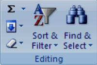
2. On the Home tab, in the Editing group, click Sort & Filter, and then click Filter.

Filter buttons appear beside each column heading as shown below:

3. Click the arrow in the column header and do one of the following:
To select from a list of text values
1. In the list of text values, select or clear one or more text values to filter by.
2. The list of text values can be up to 10,000. If the list is large, clear Select All at the top, and then select the specific text values to filter by.
To create criteria
1. Point to Text Filters and then click one of the comparison operator such as =, >, <, >=, <=, and <> commands, or click Custom Filter.
2. For example, to filter by text that begins with a specific character, select Begins With, or to filter by text that has specific characters anywhere in the text, select Contains.
3. In the Custom AutoFilter dialog box, in the box on the right, enter text or select the text value from the list.

For example, to filter by text that begins with the letter J, enter "J" or to filter by text that has "bell" anywhere in the text, enter bell.

If you need to find text that shares some characters but not others, use a wildcard character. `Wild characters and their usage are shown in the table below:

Use	To find
? (question mark)	Any single character. For example, sm?th finds "smith" and "smyth".
* (asterisk)	Any number of characters. For example, *east finds "Northeast" and "Southeast".
~ (tilde) followed by ?, *, or ~	A question mark, asterisk, or tilde. For example, fy06~? finds "fy06?".

4. Optionally, filter by one more criteria by doing one of the following:
1. To filter the table column or selection so that both criteria must be true, select And.
2. To filter the table column or selection so that either or both criteria can be true, select Or.
3. In the second entry, select a comparison operator, and then in the box on the right, enter text or select a text value from the list.
5. Click Ok.

Filtering Numbers

Range of cells

1. Select a range of cells containing numeric data.
2. Repeat step 3, 3a and 3b above.
Create criteria
1. Point to Number Filters and then click one of the comparison operator commands or click Custom Filter.
For example, to filter by a lower and upper number limit, select Between.
2. In the Custom AutoFilter dialog box, in the box or boxes on the right, enter numbers or select numbers from the list.
For example, to filter by a lower number of 25 and an upper number of 50, enter 25 and 50.
3. Optionally, filter by one more criteria by repeating step four above.

Filtering Dates or Times

Range of cells

1. Select a range of cells containing numeric data.
2. On the Home tab, in the Editing group, click Sort & Filter, and then click Filter.
3. Click the arrow in the column header.
Select from a list of dates or times
1. In the list of dates or times, select or clear one or more dates or times to filter by.
2. By default, all dates in the range of cells or table column are grouped by a hierarchy of years, months, and days. Selecting or clearing a higher level in the hierarchy selects or clears all nested dates below that level. For example, if you select 2006, months are listed below 2006, and days are listed below each month.
Create criteria
3. Point to Date Filters and then do one of the following:
For a common filter based on a comparison operator;
4. Click one of the comparison operator commands (Equals, Before, After, or Between) or click Custom Filter.
5. In the Custom AutoFilter dialog box, in the box on the right, enter a date or time, select a date or time from the list, or click the Calendar button to find and enter a date. For example, to filter by a lower and upper date or time, select Between.
6. For example, to filter by an earlier date of "3/6/2007" and a later date of "6/12/2007", enter 3/6/2007 and 6/12/2007. Dynamic filter where the criteria can change when you reapply the filter;
7. Click one of the pre-defined date commands. For example, to filter all dates by the current date, select Today, or by the following month, select Next Month.
4. Click Ok.

Filtering for Top or Bottom Numbers

Range of cells

1. Select a range of cells containing numeric data.
2. On the Home tab, in the Editing group, click Sort & Filter, and then click Filter.
3. Click the arrow in the column header.
4. Point to Number Filters and then select Top 10 and in the Top 10 AutoFilter dialog box, do the following:
1. In the box on the left, click Top or Bottom.
2. In the box in the middle, enter a number between 1 and 500.
3. In the box on the right, do one of the following:
1. To filter by number, click Items.
2. To filter by percentage, click Percent.
5. Click Ok.

Filtering by Selection

You can quickly filter data with criteria that is equal to the contents of the active cell.

1. In a range of cells or table column, right click a cell containing the value, colour, font colour, or icon you want to filter by.
2. Click Filter, and then do one of the following:
1. To filter by text, number, or date or time, click Filter by Selected Cell's Value.
2. To filter by cell colour, click Filter by Selected Cell's Color.
3. To filter by font colour, click Filter by Selected Cell's Font Color.
4. To filter by icon, click Filter by Selected Cell's Icon.

Sorting by a Custom List in Excel

Sort by a Custom List in Microsoft Excel

You can use a custom list to sort in a user-defined order. Excel provides built-in, day-of-the-week and month-of-the year custom lists, and you can also create your own custom list.

1. Select a column of data in a range of cells, or make sure that the active cell is in a table column.
2. On the Home tab, in the Editing group, click Sort & Filter, and then click Custom Sort.
The Sort dialog box is displayed.
3. Under Column, in the Sort by or Then by box, select the column that you want to sort by a custom list.
4. Click the drop down button under Order and select Custom List.
5. In the Custom Lists dialog box, select the list that you want. Or you can type in you own list by cliking the Add button and typing; for example High, Medium, Low, separated by comma.
6. Click Ok twice.

Sort Rows

1. Select a row of data in a range of cells, or make sure that the active cell is in a table column.
2. On the Home tab, in the Editing group, click Sort & Filter, and then click Custom Sort.
The Sort dialog box is displayed.
3. Click Options.
4. In the Sort Options dialog box, under Orientation, click Sort left to right, and then click Ok.
5. Under Row, in the Sort by box, select the row that you want to sort.
6. Do one of the following:
By value
1. Under Sort On, select Values.
2. Under Order, do one of the following:
1. For text values, select A to Z or Z to A.
2. For number values, select Smallest to Largest or Largest to Smallest.
3. For date or time values, select Oldest to Newest or Newest to Oldest.
By cell colour, font colour, or cell icon
1. Under Sortn, select Cell Color, Font Color, or Cell Icon.
2. Click the arrow next to the button, and then select a cell color, font color, or cell icon.
3. Under Order, select On Left or On Right.

Sort by more than one Column or Row

You might sort by more than one column or row when you have data that you want to group by the same value in one column or row, and then sort another column or row within that group of equal values. For example, if you have a Department and Employee columns, you can first sort by Department (to group all the employees in the same department together), and then sort by name (to put the names in alphabetical order within each department).

Again, if you want to find a way of categorising employees into a seniority list when such employees have the same date of employment, consider sorting by another column beside the Date Employed column. You can sort by up to 64 columns.

For best results, the range of cells that you sort should have column headings.

1. Select the entire range of cells with two or more columns of data, or make sure that the active cell is in a table with two or more columns.
2. On the Home tab, in the Editing group, click Sort & Filter, and then click Custom Sort.
The Sort dialog box is displayed.
3. Under Column, in the Sort by box, select the first column that you want to sort.
4. Under Sort On, select the type of sort by doing one of the following:
1. To sort by text, number, or date and time, select Values.
2. To sort by format, select Cell Color, Font Color, or Cell Icon.
5. Under Order, select how you want to sort by doing one of the following:
1. For text values, select A to Z or Z to A.
2. For number values, select Smallest to Largest or Largest to Smallest
3. For date or time values, select Oldest to Newest or Newest to Oldest.
4. To sort based on a custom list, select Custom List.
6. To add another column to sort by, click Add Level button, and then repeat steps three through five.
7. To copy a column to sort by, select the entry, and then click Copy Level.
8. To delete a column to sort by, select the entry, and then click Delete Level.
You must keep at least one entry in the list that is being used in the sorting.
9. To change the order in which the columns are sorted, select an entry, and then click the Up or Down arrow to change the order.

General Issues/Problems with Sorting

If you get unexpected results when sorting your data, do the following:

>Check to see if the values returned by a formula have changed. If the data that you have sorted contains one or more formulas, the return values of those formulas can change when the worksheet is recalculated. In this case, make sure that you reapply the sort or do the sort again to get up-to-date results.

Unhide rows and columns before you sort. Hidden columns are not moved when you sort columns, and hidden rows are not moved when you sort rows. Before you sort data, it's a good idea to unhide any hidden columns and rows.

Check the locale setting. Sort orders vary by locale setting. Make sure that you have the proper locale setting in Regional Settings or Regional and Language Options in Control Panel on your computer (details of control panel setting is not covered here).

Enter column headings in only one row. If you need multiple line labels, wrap the text within the cell. Detaigls of text wrapping in cells will be covered in later posts ion this blog, it will be covered under "Editing Workbook."

Turn on or off the heading row. It's usually best to have a heading row when you sort a column to make it easier to understand the meaning of the data. By default, the value in the heading is not included in the sort operation. Occasionally, you may need to turn on or off the heading so that the value in the heading is or is not included in the sort operation. Select 'My data has headers' in the sort dialog box to exclude column headers in the sort data. Then clear 'My data has headers' to include the first row of data in the sorting because it is not a column heading.

Data Sorting in Microsoft Excel

Sorting data is an integral part of data analysis. You might want to put a list of names in alphabetical order, compile a list of product inventory levels from highest to lowest, or order rows by colours or icons. Sorting data helps you quickly visualize and understand your data better, organize and find the data that you want, and ultimately make more effective decisions. To find the top or bottom values in a range of cells or table, such as top 10 grades or bottom 5 sales amounts, use AutoFilter or conditional formatting.

Sort data in a range or table

You can sort data by text (A to Z or Z to A), numbers (smallest to largest or largest to smallest), and dates and times (oldest to newest and newest to oldest) in one or more columns. You can also sort by a custom list (such as Large, Medium, and Small) or by format, including cell colour, font colour, or icon set. Most sort operations are column sorts, but you can also sort by rows.

Sort criteria are saved with the workbook so that you can reapply the sort each time that you open the workbook for an Excel table, but not for a range of cells. If you want to save sort criteria so that you can periodically reapply a sort when you open a workbook, then it's a good idea to use a table. This is especially important for multicolumn sorts or for sorts that take a long time to create.

In Excel 2007, you can apply sort states with up to sixty-four sort conditions to sort data by, but earlier versions of Excel support sort states with up to three conditions only. To avoid losing sort state information in earlier versions of Excel when the workbook is opened in an earlier version; you may want to change the sort state to one that uses no more than three conditions.

All sort state information remains available in the workbook, even after opening in an earlier version and is applied when the workbook is opened again in Excel 2007, unless the sort state information is edited in the earlier version of Excel.

Sort Text

1. Select a column of alphanumeric data in a range of cells, or make sure that the active cell is in a table column containing alphanumeric data.
2. On the Home tab, in the Editing group, and then click Sort & Filter.
3. Do one of the following:

1. To sort in ascending alphanumeric order, click Sort A to Z.
2. To sort in descending alphanumeric order, click Sort Z to A.
Optionally, you can do a case-sensitive sort.
4. On the Home tab, in the Editing group, click Sort & Filter, and then click Custom Sort.
5. In the Sort dialog box, click Options.
6. In the Sort Options dialog box, select Case sensitive.
7. Click OK twice.

Note

1. Ensure that all data is stored as text. If the column that you want to sort contains numbers stored as numbers and numbers stored as text, then you need to format them all as text. If you do not, the numbers stored as numbers are sorted before the numbers stored as text.
2. To format all of the selected data as text, on the Home tab, in the Font group, click the Format Cell Font button, click the Number tab, and then under Category, click Text.
3. Remove any leading spaces before sorting the data. In some cases, data imported from another application might have leading spaces inserted before data.

Sort Numbers

1. Select a column of numeric data in a range of cells, or make sure that the active cell is in a table column containing numeric data.
2. On the Home tab, in the Editing group, click Sort & Filter, and then do one of the following:
1. To sort from low numbers to high numbers, click Sort Smallest to Largest.
2. To sort from high numbers to low numbers, click Sort Largest to Smallest.
Important

Check to ensure that all numbers are stored as number. If the results are not what you expected, the column might contain numbers stored as text and not as numbers. For example, negative numbers imported from some accounting systems or a number entered with a leading ' (apostrophe) are stored as text. For more information, see Convert numbers stored as text to numbers in Section five of this book.

Sort Dates or Times

1. Select a column of dates or times in a range of cells, or make sure that the active cell is in a table column containing dates or times.
2. On the Home tab, in the Editing group, click Sort & Filter, and then do one of the following:
1. To sort from an earlier to a later date or time, click Sort Oldest to Newest.
2. To sort from a later to an earlier date or time, click Sort Newest to Oldest.
Important
1. Check that dates and times are stored as dates or times. If the results are not what you expected, the column might contain dates or times stored as text and not as dates or times. For Excel to sort dates and times correctly, all dates and times in a column must be stored as a date or time serial number. If Excel cannot recognize a value as a date or time, the date or time is stored as text. You can also see Section five on how to convert dates stored as text to dates.
2. If you want to sort by days of the week, format the cells to show the day of the week. If you want to sort by the day of the week regardless of the date, convert them to text by using the TEXT function. However, the TEXT function returns a text value, and so the sort operation would be based on alphanumeric data.

Sort by Cell Colour, Font Colour or Icon

If you have manually or conditionally formatted a range of cells or table column, by cell colour or font colour, you can also sort by these colours. You can also sort by an icon set created through a conditional format.
1. Select a column of data in a range of cells, or make sure that the active cell is in a table column.
2. On the Home tab, in the Editing group, click Sort & Filter, and then click Custom Sort.
The Sort dialog box is displayed.
3. Under Column, in the Sort by box, select the column that you want to sort.
4. Under Sort On, select the type of sort.
Do one of the following:
1. To sort by cell colour, select Cell Color.
2. To sort by font colour, select Font Color.
3. To sort by an icon set, select Cell Icon.
5. Under Order, select how you want to sort.
Do one of the following:
1. To move the cell colour, font colour, or icon to the top or left, select On Top for a column sort, and On Left for a row sort.
2. To move the cell colour, font colour, or icon to the bottom or right, select On Bottom for a column sort and On Right for a row sort.
6. To specify the next cell colour, font colour, or icon to sort by, click Add Level, and then repeat steps four through five.
Make sure that you select the same column in the Then by box and that you make the same selection under Order.
7. Keep repeating steps five through six for each additional cell colour, font colour, or icon that you want included in the sort.
8. Click Ok.

Protecting a Shared Workbook

If the workbook you want to protect is shared

1. If the workbook is already shared and you want to assign a password to protect the sharing, you must first unshare the workbook by doing the following:
1. Have all other users save and close the shared workbook to avoid losing their work.
2. To keep a copy of the change history information that is usually lost when you unshare a workbook, do the following:
1. Click on the Review tab, in the Changes group, click Track Changes, and then click Highlight Changes.
2. In the When list, select All.
3. Clear the Who and Where check boxes.
4. Select the List changes on a new sheet check box, and then click OK.
5. Print the History worksheet or copy the history to another workbook.
Change history is the information that is maintained about changes made in past editing sessions of a shared workbook. The information includes the name of the person who made each change, when the change was made, and what data was changed.
2. In the shared workbook, on the Review tab, in the Changes group, click Share Workbook.
3. On the Editing tab, make sure that you are the only person listed in the 'Who has this workbook open now' list.
4. Clear the 'Allow changes by more than one user at the same time. This also allows workbook merging' check box. If this check box is not available, then you must unprotect the workbook before clearing the check box.
5. Clic Ok. When you are prompted about the effects on other users, click Yes.
If needed, give specific users access to ranges, protect worksheets, protect workbook elements, and set passwords for viewing and editing.
6. If prompted, save the workbook.

To Unprotect Workbook

1. Click on the Review tab, in the Changes group, click 'Unprotect Workbook.'
2. If you are prompted, enter the password and then click OK.