Protecting Workbook's Structure and Window

Protecting the Structure and Windows of a Workbook

You can lock the structure of a workbook to prevents users from adding or deleting worksheets or from displaying hidden worksheets in that workbook. You can also prevent users from changing the size or position of worksheet windows. Note that workbook structure and window protection applies to the entire workbook.

To prevent a user from accidentally or deliberately changing, moving, or deleting important data, you can protect certain worksheet or workbook elements, with or without a password.

NOTE: a. Workbook and worksheet element protection should not be confused with workbook-level password security. Element protection cannot protect a workbook from users who have malicious intent.
b. If the workbook is already shared and you want to assign a password to protect the sharing, you must first un-share the workbook.

Protect worksheet or workbook elements

When you protect a worksheet, all cells on the worksheet are locked by default, and users cannot make any changes to a locked cell. For instance, they cannot insert, modify, delete, or format data in a locked cell. You can, however, specify which elements users will be allowed to change when you protect the worksheet.

Steps to Protect Worksheet Elements

1. Select the worksheet that you want to protect.
2. To unlock any cells or ranges that you want other users to be able to change:
1. Select each cell or range that you want to unlock.
2. Click on the Home tab, in the Cells group, click Format, and then click Format Cells.
3. On the Protection tab, clear the Locked check box, and then click OK.
3. To hide any formulas that you don't want to be visible, do the following:
1. In the worksheet, select the cells that contain the formulas that you want to hide.
2. Click on the Home tab, in the Cells group, click Format, and then click Format Cells.
3. On the Protection tab, select the Hidden check box, and then click OK.
4. Now to protect the worksheet proper; click on the Review tab, in the Changes group, click Protect Sheet.
5. In the 'Allow all users of this worksheet to' list, select the elements that you want users to be able to change.
6. In the 'Password to unprotect sheet' box, type a password for the sheet, click Ok.
7. Retype the password to confirm it and click Ok.

Protect workbook elements

1. Click on the Review tab, in the Changes group, click Protect Workbook.
2. Then click Protect structure and window.
3. Under 'Protect workbook for', do any of the following:

1. To protect the structure of a workbook, select the Structure check box.
2. To keep workbook windows in the same size and position each time the workbook is opened, select the Windows check box.
4. Note that STRUCTURE prevents unauthorized users from; viewing worksheets that you have hidden, deleting, hiding, or changing the names of worksheets, inserting new worksheets or chart sheets, moving or copying worksheets to another workbook. In PivotTable reports; prevents them from displaying the source data for a cell in the data area, or displaying page field pages on separate worksheets. For SCENARIOS; it prevents them from creating a scenario summary report or recording new macros. The WINDOWS option prevents unauthorized users from changing the size and position of the windows for the workbook when the workbook is opened, moving, resizing, or closing the windows. But Users will be able to hide and unhide windows.

Workbook elements

5. To prevent other users from removing workbook protection, in the Password (optional) box, type a password, click Ok, and then retype the password to confirm it.

Connecting to Access Data from Excel

Connect to Access Data from Excel

To bring refreshable Access data into Excel, you can create a connection, to the Access database and retrieve all of the data from a table or query. The main benefit of connecting to Access data is that you can periodically analyse this data in Excel without repeatedly copying or exporting the data from Access. After you connect to the data, you can also automatically refresh (or update) your Excel workbooks from the original Access database whenever the database is updated with new information. For example, you may want to update an Excel summary budget report that you distribute every month so that it contains the current month's data.

1. From Excel window, click the cell where you want to put the data from the Access database.
2. Click on the Data tab, in the Get External Data group, click From Access.
3. In the Look in list, locate and double-click the Access database that you want to import.
4. In the Select Table dialog box, click the table or query that you want to import, and then click Ok.
5. In the Import Data dialog box, do the following:
1. Under Select how you want to view this data, do one of the following:
1. To view the data as a table, select Table.
2. To view the data as a PivotTable report, select PivotTable report.
3. To view the data as a PivotChart and PivotTable report, select PivotChart and PivotTable report.
2. Under Where do you want to put the data? Do one of the following:
1. To return the data to the location that you selected, click Existing worksheet.
2. To return the data to the upper-left corner of the new worksheet, click New worksheet.
6. Click Ok.

 

Copy Access Data into Excel

From Microsoft Access, you can copy data from a datasheet view and then paste the data into an Microsoft Excel worksheet. Additionally, you can take the following steps to copy data from Microsoft Access to Microsoft Excel:

1. Start Access, and then open the table, query, or form that contains the records that you want to copy.
2. Click on the Home tab, click View, and then click Datasheet View.
3. Select the records that you want to copy. If you want to select specific columns, drag across adjacent column headings.

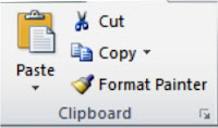
4. On the Home tab, in the Clipboard group, click Copy.
5. Start Excel, and then open the worksheet that you want to paste the data into.
6. Click in the upper-left corner of the worksheet area where you want the first field name to appear.
7. To ensure that the copied records do not replace existing records, make sure that the worksheet has no data below or to the right of the cell that you click.
8. Click on the Home tab, in the Clipboard group, click Paste.

Practical Export of Data Between Access and Excel

Operation to Export Data Between Access and Excel

In my previous post I showed the several ways to exchange data between Microsoft Access and Microsoft Excel. whether to bring data into Excel from Access, to bring data into Access from Excel; you can take the following steps to accomplish it.

1. If you are working in Microsoft Access and want to export data to Microsoft Excel, open the source database.
2. In the Navigation Pane, select the object that contains the data that you want to export. (It can be a table, a query, or a form).
3. Review the source data to ensure that it does not contain any error indicators or error values. (If there are any errors, you must resolve them before you export the data to Excel. Otherwise, errors can occur during the export operation, and null values might be inserted into fields).
4. If the source object is a table or a query, decide whether you want to export the data with or without its formatting.
5. Choose the destination workbook and file format.
6. During the export operation, Access prompts you to specify the name of the destination workbook. The workbook is then created if it does not exist. But if it exists, it is overwritten if the data, including the formatting is exported, otherwise; if the data, but not the formatting is exported, the workbook is not overwritten, instead a new worksheet is added to the workbook, and is given the name of the object from which the data is being exported.
7. If the destination Excel workbook is open, close it before you continue.

Export the Data

8. In the source database, if you want to export only a portion of a table, query, or form, open the object and select the records you want.


9. On the External Data tab, in the Export group, click Excel.
10. In the Export - Excel Spreadsheet dialog box, accept the suggested name for the Excel workbook or enter another name.
11. In the File Format box, select the file format that you want.
12. If you are exporting a table or a query, and you want to export formatted data, select 'Export data with formatting and layout'.
13. To view the destination Excel workbook after the export operation is complete, select the 'Open the destination file after the export operation is complete' check box.
14. If the source object is open, and if you selected one or more records in the view before starting the export operation, you can select Export only the selected records. However, if you want to export all of the records displayed in the view, leave this check box cleared.

View that dialog box below.

15. Click Ok.

If the export operation fails due to an error, Access displays a message that describes the cause of the error. Otherwise, Access exports the data to the destination workbook in Excel. Access then displays a dialog box in which you can create a specification that uses the details from the export operation.

 

 

Save the Export Specification

1. Click Yes if you want to save the details of the export operation for future use. This helps you repeat the same export operation in the future without having to go through the entire steps in the wizard each time.
2. In the Save as box, type a name for the export specification.
3. If you want to perform the operation at fixed intervals (such as weekly or monthly), select the Create Outlook Task check box.
4. Click Save Export.

If Outlook is installed, Access starts it immediately. This creates a Microsoft Office Outlook 2007 task that lets you run the specification by clicking a button.

5. In Outlook, review and modify the task settings (such as Due date and Reminder).
6. To make the task recur, click Recurrence. This dialog box below shows the task scheduler with some typical settings.
7. Click Save and Close.

Run the Saved Task

1. In the Outlook Navigation Pane, click Tasks, and then double-click the task that you want to run.
2. On the Task tab, in the Microsoft Office Access group, click Run Import.
3. In Excel, open the destination workbook, and then verify that all of the data were copied into the correct cells.

Exchange Data Between Excel and Access

How to Exchange Data Between Microsoft Excel and Access

There are several ways to exchange data between Microsoft Office Access and Microsoft Office Excel. To bring data into Excel from Access, you can copy data from an Access datasheet and paste it into an Excel worksheet, connect to an Access database from an Excel worksheet, or export Access data into an Excel worksheet.

To bring data into Access from Excel, you can copy data from an Excel worksheet and paste it into an Access datasheet, import an Excel worksheet into an Access table, or link to an Excel worksheet from an Access table.

The word IMPORT has two different meanings between Excel and Access. In Excel, the word import means to make a permanent connection to data that can be refreshed. In Access, the word import means to bring data into Access once, but without a data connection. You CANNOT save an Excel workbook as an Access database. Neither Excel nor Access provides functionality to create an Access database from Excel data.

Export Access Data to Excel

You may want to work with Access data in an Excel workbook in order to take advantage of the data analysis and charting features, the flexibility in data arrangement and layout, or the many functions that are not available in Access. You can copy data from a Microsoft Office Access 2007 database into a worksheet by exporting a database object to a Microsoft Office Excel 2007 workbook. You do this by using the Export Wizard in Office Access 2007.

By using the Export Wizard in Access, you can export an Access database object, such as a table, query, or form, or selected records in a view into an Excel worksheet. When you perform an export operation, you can save the details for future use, and even schedule the export operation to run

Scenarios for Exporting Access Data to Excel

The following are common situations for exporting data from Access to Excel:

1. Your department or workgroup uses both Access and Excel to work with data. You store the data in Access databases, but you use Excel to analyze the data and to distribute the results of your analysis. Your team currently exports data to Excel when they need to, but if you would like to make this process more efficient, you might need to export date between the two office applications.
2. Another scenario may be that you are a long-time user of Access, but your manager prefers to view reports in Excel. At regular intervals, you do the work of copying the data into Excel, but you would like to automate this process to save yourself time, so you would need to export data.
   Note
1. To export data from Access to Excel, you must be working in Access. Excel does not provide any mechanism for importing data from an Access database. Again, you cannot save an Access database or table as an Excel workbook by using the Save As command of Access. You can only use the Save As command of Access to save an Access object in the current database as another Access database object.
2. You can export a table, query, or form. You can also export selected records in a view.
3. You cannot export macros, modules, or reports to Excel. When you export a form or datasheet that contains subforms or subdatasheets, only the main form or datasheet is exported. You must repeat the export operation for each subform and subdatasheet that you want to view in Excel.
4. You can only export one database object in a single export operation. However, you can merge the data in multiple worksheets in Excel after completing the individual export operations.

 

How Microsoft Excel Fills in Series of Numbers, Dates, etc.

/* Google Analytic Tracking Code*/ /* End of Google Analytic Tracking Code*/

How to Fill in Series of Numbers, Dates, or other built-in Series Items in Microsoft Excel

In Microsoft Excel, you can Use the fill handle to quickly fill cells in a range with a series of numbers or dates or with a built-in series for days, weekdays, months, or years. The following steps will enable fill such series into Excel cell:

1. Type in the starting value for the series in the first cell.
2. Type a value in the next cell to establish a pattern.
• For instance, if you want the series 1, 2, 3, 4, 5..., type 1 and 2 in the first two cells. If you want the series 2, 4, 6, 8..., type 2 and 4. If you want the series 2, 2, 2, 2..., you can leave the second cell blank.
3. Select the cells that contain the both starting values you have just typed.
4. Point the mouse to the lower-right corner of the selected cell(s) and drag the fill handle across the range that you want to fill.

5. To fill in increasing order, drag downwards or to the right. To fill in decreasing order, drag upwards or to the left.
• You can also specify the type of series by using the right mouse button to drag the fill handle over the range and then clicking the appropriate command on the shortcut menu. For instance, if the starting value is a date like JAN-2002, click Fill Months in order to have FEB-2002, MAR-2002, and so on; or click Fill Years in order to have JAN-2003, JAN-2004, and so on.
• If the selection contains numbers, you can control the type of series that you want to create. For instance, click Fill Series in order to have serial numbering in ascending order, or click Formatting Only in order to copy only the format of the selected cell(s).

Other examples of data that Microsoft Excel can automatically fill are shown in the table below: When you fill a series, the selections are extended as shown in the following table. Items separated by commas are in placed in individual adjacent cells.

Initial selection	Extended series
1, 2, 3	4, 5, 6,...
9:00	10:00, 11:00, 12:00,...
Mon	Tue, Wed, Thu,...>
Monday	Tuesday, Wednesday, Thursday,...
Jan	Feb, Mar, Apr,...
Jan, Apr	Jul, Oct, Jan,...
Jan-99, Apr-99	Jul-99, Oct-99, Jan-00,...
15-Jan, 15-Apr	15-Jul, 15-Oct,...
1999, 2000	2001, 2002, 2003,...
1-Jan, 1-Mar	1-May, 1-Jul, 1-Sep,...
Qtr3 (or Q3 or Quarter3)	Qtr4, Qtr1, Qtr2,...
text1, textA	text2, textA, text3, textA,...
1st Period	2nd Period, 3rd Period,...
Product 1	Product 2, Product 3,...

Fill Data in Cells with Fill Handle

Use the Fill Handle to Fill Data

You can use the Fill command to fill data into worksheet cells. You can also have Excel automatically fill series of numbers, number and text combinations, dates, or time periods, based on a pattern that you establish. However, to quickly fill in several types of data series, you can select cells and drag the fill handle. The fill handle is the small black square that usually display when the mouse pointer is placed on at the lower-right corner of the cell-pointer.

Fill data into adjacent cells

1. Select the cell(s) that contain the data that you want to fill into adjacent cells.
2. Point the mouse to the lower-right corner of the selected cell(s). The mouse pointer changes to a small black cross.
3. Drag the fill handle (small black cross) across the cells that you want to fill.
4. After you drag the fill handle, the Auto Fill Options button appears so that you can choose how the selection is filled. For instance, you can choose to fill just cell formats by clicking Fill Formatting Only, or you can choose to fill just the contents of a cell by clicking Fill Without Formatting.

5. To quickly fill a blank cell with the contents of the cell above it; press CTRL+D, to fill to the right of that cell, press CTRL+R.
6. You can suppress AutoFill by holding down CTRL while you drag the fill handle of a selection of two or more cells. The selected values are then copied to the adjacent cells, and Excel does not extend a series.

NOTE that if you drag the fill handle up or to the left of a selection and stop in the selected cells without going past the first column or the top row in the selection, Excel deletes the data within the selection. You must drag the fill handle out of the selected area before releasing the mouse button.

Specifying Response to Invalid Data Entry

How to Specify a Response to Invalid Data Entry in Microsoft Excel

In my last post, I showed how to make data entry easier, or limit entries to certain items that you define and ensure the correct data is entered in Excel worksheet. Additionally, you can specify how you want Microsoft Office Excel to respond when invalid data is entered. Take these the following steps to create Response to Invalid Data Entry in Excel:

• First, you have to create a list of valid entries for the drop-down list, so type the entries in a single column or row without blank cell as can be seen in this picture below.

• You can sort the data in the order that you want it to appear in the drop-down list.
• If you want to use another worksheet, type the list on that worksheet, and then define a name for the list. (Click Defining Name Reference to read my post on that).
  1. Select the cell where you want the drop-down list.
  2. Click on the Data tab, in the Data Tools group, click Data Validation. The Data Validation dialog box will be displayed.
  3. Click the Settings tab.
  4. In the Allow box, click List.
  5. To specify the location of the list of valid entries, do one of the following:
  • If the list is in the current worksheet, enter a reference to your list in the Source box. For example, enter =Depts or =$C$5:$C$25.
  • If the list is on a different worksheet, enter the name that you defined for your list in the Source box.
  6. Make sure that the In-cell drop-down check box is selected.
  7. 2) Click the Error Alert tab, and make sure that the "Show error alert after invalid data" is entered check box is selected.
  8. 3) Select one of the following options for the Style box:
  • To display an information message that does not prevent entry of invalid data, click Information.
  • To display a warning message that does not prevent entry of invalid data, click Warning.
  • To prevent entry of invalid data, click Stop.
  9. Type the title and text for the message (up to 225 characters).
  10. Click Ok.

Creating Drop-Down List in Excel

Create a Drop-Down List from a range of cells

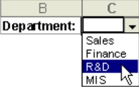
In Microsoft Excel, to make data entry easier, or to limit entries to certain items that you define and ensure the correct data is entered, you can create a drop-down list of valid entries that is compiled from cells elsewhere in the workbook. When you create a drop-down list for a cell, it displays an arrow in that cell. To enter information in the cell, click the arrow, and then click the entry that you want.

In this way you don't have to type the data again and again at every occurrence, you simply select it from the drop-down list as picking items from a list. The Data Validation command in the Data Tools group on the Data tab can also be used to achieve this.

• To create a list of valid entries for the drop-down list, type the entries in a single column or row without blank cell as can be seen in this picture below.

• You can sort the data in the order that you want it to appear in the drop-down list.
• If you want to use another worksheet, type the list on that worksheet, and then define a name for the list. (Click Defining Name Reference to read my post on that).
  1. Select the cell where you want the drop-down list.
  2. Click on the Data tab, in the Data Tools group, click Data Validation. The Data Validation dialog box will be displayed.
  3. Click the Settings tab.
  4. In the Allow box, click List.
  5. To specify the location of the list of valid entries, do one of the following:
  • If the list is in the current worksheet, enter a reference to your list in the Source box. For example, enter =Depts or =$C$5:$C$25.
  • If the list is on a different worksheet, enter the name that you defined for your list in the Source box.
  6. Make sure that the In-cell drop-down check box is selected.
  7. Click Ok.

Create a Calculated Column in Excel

How to Create a Calculated Column in Excel

One of the most beautiful things about Microsoft Excel is the ability to automatically perform calculation on data in tables. You can create a calculated column that uses a single formula that adjusts for each row, i.e. as you enter more data in the succeeding rows, the formula automatically extends to them without you having to enter the formula over and over again. You only need to enter a formula only once and don't need to use the Fill or Copy command. NOTE that this will only work in an Excel table not on range of data. To learn how to create a Table in Excel, read my earlier post on Creating Tables in Excel. Take the following steps to create Calculated Column:

1. Click a cell in a blank table column that you want to turn into a calculated column.
2. Type the formula that you want to use.
3. The formula that you typed is automatically filled into all cells of the column — above as well as below the active cell.

Insert a Table Row or Column

Select the Table and do one of the following:

• To insert one or more table rows, select one or more table rows above which you want to insert one or more blank table rows.
• If you select the last row, you can also insert a row above or below the selected row.
• To insert one or more table columns, select one or more table columns to the left of which you want to insert one or more blank table columns.
• If you select the last column, you can also insert a column to the left or to the right of the selected column.

1. On the Home tab, in the Cells group, click the arrow next to Insert.
2. Do one of the following:
   • To insert table rows, click Insert Table Rows Above.
   • To insert a table row below the last row, click Insert Table Row Below.
   • To insert table columns, click Insert Table Columns to the Left.
   • To insert a table column to the right of the last column, click Insert Table Column to the Right.
3. You can also right-click one or more table rows or table columns, point to Insert on the shortcut menu, and then select what you want to do from the list of options.

Delete Rows or Columns in a Table

1. Select one or more table rows or table columns that you want to delete.
2. On the Home tab, in the Cells group, click the arrow next to Delete, and then click Delete Table Rows or Delete Table Columns.

Delete a Row or Column

1. To delete a row or column, select the row or column you want to delete.
2. On the Home tab, in the Cells group, click Delete or press DELETE key on the keyboard.

Convert a Table to a Range of Data

1. Click anywhere in the table. This displays the Table Tools, adding the Design tab.
2. On the Design tab, in the Tools group, click Convert to Range.

You can also right-click the table, point to Table, and then click Convert to Range.

Delete a Table

1. On a worksheet, select a table.
2. Press DELETE on the keyboard.

 

How to Create Table in Excel

Creating a Table in Microsoft Excel

When you create a table in Microsoft Office Excel, you can manage and analyze the data in that table independently of data outside of the table. For example, you can filter table columns, add a row for totals, apply table formatting, and publish a table to a server that is running Microsoft Windows SharePoint Services 3.0.

When you don't need a table anymore, you can remove it by converting it back to a range or you can delete it.

To Create a Table take the following steps:

1. On a worksheet, select the range of empty cells or data that you want to make into a table.
2. On the Insert tab, in the Tables group, click Table.
3. If the selected range contains data that you want to display as table headers, select the 'My table has headers' check box.

Table headers display default names that you can change if you don't select the 'My table has headers' check box. After you create a table, the Table Tools become available, and a Design tab is displayed. You can use the tools on the Design tab to customize or edit the table. After you create a table, the Table Tools become available, and a Design tab is displayed. You can use the tools on the Design Tab to customize or edit the table.

 

Introduction to Microsoft Excel Tables

Microsoft Excel Tables

To make managing and analyzing a group of related data easier, you can turn a range of cells into a Microsoft Office Excel table (previously known as an Excel list in earlier versions). A table is a series of rows and columns that contains related data that is managed independently from the data in other rows and columns on the worksheet.

By default, every column in the table has filtering enabled in the header row so that you can filter or sort your table data quickly. You can add a total row, which is a special row in a list that provides a selection of aggregate functions useful for working with numerical data to your table that provides a drop-down list of aggregate functions for each total row cell. A sizing handle in the lower-right corner of the table allows you to drag the table to the size that you want just like Microsoft Office Word table.

To manage several groups of data, you can insert more than one table in the same worksheet. However, you cannot create a table in a shared workbook.

You can use the following features to manage table data:

Sorting and filtering. Filter drop-down lists are automatically added in the header row of a table. Then you can sort tables in various orders and options, or you can create a custom sort order. You can also filter tables to show only the data that meets the criteria you set. For more information on sorting and filtering data, see Data Sorting and Filtering in Section Two of this book.

Formatting table data. You can quickly format table data by applying a predefined or custom table style. You can also choose Quick Styles options to display a table with or without a header or a totals row, to apply row or column banding to make a table easier to read, or to distinguish between various columns in the table. For more information on how to format table data, see Formatting Worksheet in Section Five of this book.

Inserting and deleting table rows and columns. You can use one of several ways to add rows and columns to a table. You can quickly insert table rows and table columns anywhere that you want. You can as well delete rows and columns as needed. You can also quickly remove rows that contain duplicate data from a table.

Using a calculated column. To use a single formula that adjusts for each row in a table, you can create a calculated column. A calculated column automatically expands to include additional rows so that the formula is immediately extended to those rows.

Displaying and calculating table data totals. You can quickly total the data in a table by displaying a totals row at the end of the table and then using the functions that are provided in drop-down lists for each totals row cell. Exporting to a SharePoint list. You can export a table to a SharePoint list so that other people can view, edit, and update the table data.

How to Enter the same Data into Several Cells at Once

Enter the same Data into Several Cells at Once

This procedure enables you to automate data entering into cells into Microsoft Excel cells and speed up your work

1. Select the cells into which you want to enter the same data. The cells do not have to be adjacent.
2. In the active cell, type the data, and then press CTRL+ENTER.
3. You can also enter the same data into several cells by using the fill handle to automatically fill data in worksheet cells. See details below in this section for more information.

Enter the same data on Other Worksheets

If you already entered data on one worksheet, you can quickly fill this data into corresponding cells on other worksheets.

1. Click the tab of the worksheet that contains the data. Then hold down CTRL while you click the tabs of other worksheets into which you want to fill the data.
2. In the source worksheet, select the cells that contain the data that you entered.

3. On the Home tab, in the Editing group, click Fill, and then click Across Worksheets.

How to Enter Numbers as Texts in Microsoft Excel

You might need to enter numbers that are not required for calculation, for instance phone numbers, employee IDs, customer IDs, Registration numbers, etc. When these numbers are has leading zeros or preceded by zero, Excel would remove the leading zeros after the texts have been entered. In order to retain the leading zeros, precede the numbers with an apostrophe ( ' ) and such numbers will be stored as texts and cannot be calculated by Excel.

How to Enter Data in Excel Worksheet

Enter data manually in worksheet cells

You can enter numbers (with or without fixed decimal points), text, dates, or times in one cell, in several cells at once, or on more than one worksheet. However, when a worksheet is protected by you or someone else to prevent data from being changed accidentally, you may be able to select cells to view the data, but you won't be able to type information in cells that are locked. In most cases, a protected worksheet should not be unprotected unless you have permission to do so from the person who created it.

To Enter numbers or text

1. On the worksheet, click a cell.
2. Type the numbers or text that you want, and then press ENTER or TAB.
3. To start entering data on a new line within a cell, enter a line break by pressing ALT+ENTER.

By default, pressing ENTER moves the selection down one cell, and pressing TAB moves the selection one cell to the right. You cannot change the direction of movement for the TAB key, but you can specify a different direction for the ENTER key.

How to Change the Direction for the ENTER key

1. Click the MS Office Button or File, and then click Excel Options.
2. In the Advanced category, under Edit, select the After pressing Enter, move selection check box.
3. Then click the direction that you want in the Direction box.
4. Click Ok.

NOTE: A cell may display ##### when it contains data that has a number format that is wider than the column width, or the contents may simply be truncated. To see all text, you must increase the width of the column. You can display multiple lines of text inside a cell by wrapping the text. (more details on formatting worksheet with be in subsequent posts). In order to expand the width of column to accommodate the longest entry; use the mouse to double-click the right border of the column heading.

How to Enter Dates or Times In Microsoft Excel

On the worksheet, click a cell, type a date or time as follows:

1. For a date, use a forward slash or a hyphen to separate the parts of a date; for example, type 9/5/2002 or 5-Sep-2002.
2. To enter the current date, press CTRL+; (CTRL+semicolon).
3. For a time that is based on the 12-hour clock, type a space, and then type a or p after the time; for example, 9:00 p. Otherwise, Excel enters the time as AM.
4. To enter the current time, press CTRL+SHIFT+; (CTRL+SHIFT+semicolon).
5. To enter a date or time that stays current when you reopen a worksheet, you can use the TODAY and NOW functions for instance type =Today() or type =Now() and press ENTER.
6. If you want to use the default date or time format, click the cell that contains the date or time, and then press CTRL+SHIFT+# or CTRL+SHIFT+@.

How Do I Enter Data into a Cell?

Entering Data into a Cell

You can enter numbers, text, dates, times or formula in a cell, in several cells at once, or on more than one worksheet. To work effectively in Excel, you must be able to move around the workbook. The various ways to move around a worksheet has been treated above in this section.

To enter data into a cell, simply place the cell pointer on the desired cell and type the data. Microsoft Excel has various ways of assisting users to enter data into worksheet; some of such ways are treated in the succeeding posts.

How to Automatically Repeat Items Already Entered in the Column.

If the first few characters that you type in a cell match an existing entry in that column, Excel automatically enters the remaining characters for you. However, only those entries that contain text or a combination of text and numbers that Excel automatically completes. Entries that contain only numbers, dates, or times are not automatically completed.

Do one of the following:

1. To accept a proposed entry, press ENTER key. The completed entry exactly matches the pattern of uppercase and lowercase letters of the existing entry.
2. To replace the automatically entered characters, continue typing.
3. To delete the automatically entered characters, press BACKSPACE.

If you don't want entries that you type to be completed automatically, you can turn off this option by taking the following steps:

1. Click the Microsoft Office Button File menu (depending on the Office version you have), and then click Excel Options.
2. Click Advanced, and then under Editing options, clear or select the Enable AutoComplete for cell values check box to turn automatic completion of cell values on or off.

NOTE: Microsoft Excel bases the list of potential AutoComplete entries on the column that contains the active cell. Entries that are repeated within a row are not automatically completed.

Views in Microsoft Excel

Various Views in Microsoft Excel

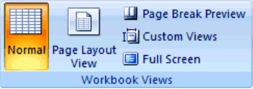
Before you print a Microsoft Office Excel worksheet that contains large amounts of data or charts, you can quickly fine-tune it in the new Page Layout view to achieve professional-looking results. In this view, you can change the layout and format of data the way that you can in Normal view. But you can also use the rulers to measure the width and height of the data, change the page orientation, add or change page headers and footers, set margins for printing, and hide or display row and column headers.

Page Layout view is useful to get your data ready for printing. Page breaks are more easily adjusted in Page Break Preview view. For an exact preview of how the data will be printed, you can preview the worksheet pages in Print Preview view.

Select scaling options in Normal View

1. Click the worksheet that you want to change its view.
2. Click on the View tab, in the Workbook Views group, click Page Layout View or Page Break Preview or Full Screen.

You can also click any of these views on the status bar.

Freeze or Lock Rows and Columns

How Do I Freeze or Lock Rows and Columns in Excel?

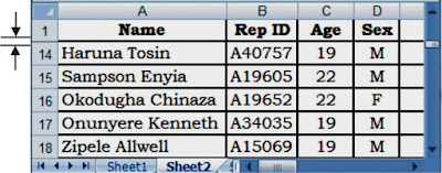
You can view two areas of a worksheet and lock rows or columns in one area by freezing or splitting panes. When you freeze panes, you select specific rows or columns that remain visible and immovable when scrolling in the worksheet. For example, you would freeze panes to keep row and column labels visible as you scroll, as shown in the example below where row 1 is frozen.

When you split panes, you create separate worksheet areas that you can scroll within, while rows or columns in the non-scrolled area remain visible.

Steps to Freeze Panes to lock specific rows or columns

On the worksheet, do one of the following:

1. To lock rows, select the row below where you want the split to appear.
2. To lock columns, select the column to the right of where you want the split to appear.
3. To lock both rows and columns, click the cell below and to the right of where you want the split to appear.

On the View tab, in the Window group, click Freeze Panes, and then click the option that you want.

Split panes to lock rows or columns in separate worksheet areas:

1. To split panes, point to the split box at the top of the vertical scroll bar or at the right end of the horizontal scroll bar.
2. When the mouse pointer changes to a split pointer or , drag the split box down or to the left to the position that you want at the centre of the worksheet.
   
3. To remove the split, double-click any part of the split bar that divides the panes.

This would enable you view or compare different parts of worksheet that are far apart in close range. For instance, you can compare data in column B with data in column AZ at the same time.

Access The Ribbon Bar Using Keyboard

Keyboard Access To The Ribbon Bar

To acess the Ribbon Bar using the keyboard, take the following steps:

1. Press ALT
2. The KeyTips are displayed over each feature that is available in the current view.
3. Press the letter that appears in the KeyTip over the feature that you want to use.
4. Depending on which letter you press, additional KeyTips may appear. For example, if the Home tab is active and you press I, the Insert tab is displayed, along with the KeyTips for the groups on that tab.
   
5. Continue pressing letters until you press the letter of the command or control that you want to use. In some cases, you must first press the letter of the group that contains the command.
6. To cancel the action that you are taking and hide the KeyTips, press ALT.

Other Shortcut Keys in Microsoft Excel

This articles describes all the other useful shorcut keys in Microsoft Excel that can enable you perform many functions quickly while working in Microsoft Excel. They keys include the Shift Key combine with the Arrow keys, or combining Alt key with the Enter Key and combining Ctrl, Shift with Enter keys and many other key combinantions.

KEYS	DESCRIPTION
ARROW KEYS	The Arrow keys move one cell up, down, left, or right in a worksheet. CTRL+ARROW keys move to the edge of the current data region in a worksheet. Note that data region is a range of cells that contains data and that is bounded by empty cells or datasheet borders. SHIFT+ARROW key extends the selection of cells by one cell. CTRL+SHIFT+ARROW key extends the selection of cells to the last nonblank cell in the same column or row as the active cell, or if the next cell is blank, extends the selection to the next nonblank cell. LEFT ARROW or RIGHT ARROW key selects the tab to the left or right when the ribbon is selected. When a submenu is open or selected, these arrow keys switch between the main menu and the submenu. When a ribbon tab is selected, these keys navigate the tab buttons. DOWN ARROW or UP ARROW selects the next or previous command when a menu or submenu is open. When a ribbon tab is selected, these keys navigate up or down the tab group. In a dialog box, arrow keys move between options in an open drop-down list, or between options in a group of options. DOWN ARROW or ALT+DOWN ARROW opens a selected drop-down list.
BACKSPACE	The Backspace key deletes one character to the left in the Formula Bar. It also clears the content of the active cell. In cell editing mode, it deletes the character to the left of the insertion point.
DELETE	The Delete key removes the cell contents from selected cells without affecting cell formats or comments. In cell editing mode, it deletes the character to the right of the insertion point.
END	The End key moves to the cell in the lower-right corner of the window when SCROLL LOCK is turned on. Also selects the last command on the menu when a menu or sub-menu is visible. CTRL+END move to the last cell on a worksheet, in the lowest used row of the rightmost used column. If the cursor is in the formula bar, CTRL+END move the cursor to the end of the text. CTRL+SHIFT+END extend the selection of cells to the last used cell on the worksheet (lower-right corner). If the cursor is in the formula bar, CTRL+SHIFT+END select all text in the formula bar from the cursor position to the end—this does not affect the height of the formula bar.
ENTER	The Enter key completes a cell entry from the cell or the Formula Bar, and selects the cell below (by default). In a data form, it moves to the first field in the next record. Opens a selected menu (press F10 to activate the menu bar) or performs the action for a selected command. In a dialog box, it performs the action for the default command button in the dialog box (the button with the bold outline, often the OK button). ALT+ENTER starts a new line in the same cell. CTRL+ENTER fills the selected cell range with the current entry. SHIFT+ENTER completes a cell entry and selects the cell above.
ESC	The ESC key cancels an entry in the cell or Formula Bar. It closes an open menu or sub-menu, dialog box, or message window. It also closes full screen mode when this mode has been applied, and returns to normal screen mode to display the Ribbon and status bar again.
HOME	The Home key moves to the beginning of a row in a worksheet. It also move to the cell in the upper-left corner of the window when SCROLL LOCK is turned on. Selects the first command on the menu when a menu or submenu is visible. CTRL+HOME move to the beginning of a worksheet. CTRL+SHIFT+HOME extend the selection of cells to the beginning of the worksheet.
PAGE DOWN	The Page Down key move one screen down in a worksheet. ALT+PAGE DOWN move one screen to the right in a worksheet. CTRL+PAGE DOWN move to the next sheet in a workbook. CTRL+SHIFT+PAGE DOWN select the current and next sheet in a workbook.
PAGE UP	The Page Up key move one screen up in a worksheet. ALT+PAGE UP move one screen to the left in a worksheet. CTRL+PAGE UP move to the previous sheet in a workbook. CTRL+SHIFT+PAGE UP select the current and previous sheet in a workbook.
SPACEBAR	In a dialog box, the Spacebar key performs the action for the selected button, or selects or clears a check box. CTRL+SPACEBAR select an entire column in a worksheet. SHIFT+SPACEBAR select an entire row in a worksheet. CTRL+SHIFT+SPACEBAR select the entire worksheet. Important. a. If the worksheet contains data, CTRL+SHIFT+SPACEBAR select the current region. Pressing CTRL+SHIFT+SPACEBAR a second time select the current region and its summary rows. Pressing CTRL+SHIFT+SPACEBAR a third time select the entire worksheet. b. When an object is selected, CTRL+SHIFT+SPACEBAR select all objects on a worksheet. ALT+SPACEBAR display the Control menu for the Microsoft Office Excel window.
TAB	The Tab key moves one cell to the right in a worksheet. Moves between unlocked cells in a protected worksheet. It also moves to the next option or option group in a dialog box. SHIFT+TAB move to the previous cell in a worksheet or the previous option in a dialog box. CTRL+TAB switche to the next tab in dialog box. CTRL+SHIFT+TAB switche to the previous tab in a dialog box.

 

F1 to F12 Function Keys: Microsoft Excel

What Do The F1 to F12 Function Keys Do in Microsoft Excel?

The following article explains all the function of the Function Key in Microsoft Excel, starting from F1 to F12 keys when used alone and when used in combination with the CTRL key, SHIFT Key and the ALT Key. You can always visit this blog for other function you may require and if the action you perform often does not have a function key for it, you can record a macro to perform it. Later on on this blog, I will post how to record a macro for such activity.

KEY	DESCRIPTION
F1	F1 Key displays the Microsoft Office Excel Help task pane. CTRL+F1 displays or hides the ribbon. ALT+F1 creates a chart of the data in the current range. ALT+SHIFT+F1 inserts a new worksheet.
F2	F2 Key edits the active cell and positions the insertion point at the end of the cell contents. It also moves the insertion point into the Formula Bar when editing in a cell is turned off. SHIFT+F2 adds or edits a cell comment. CTRL+F2 displays the Print Preview window.
F3	F3 Key displays the Paste Name dialog box. SHIFT+F3 displays the Insert Function dialog box.
F4	F4 Key repeats the last command or action, if possible. CTRL+F4 closes the selected workbook window.
F5	F5 Key displays the Go To dialog box. CTRL+F5 restores the window size of the selected workbook window.
F6	F6 Key switches between the worksheet, ribbon, task pane, and Zoom controls. In a worksheet that has been split (View menu, Manage This Window, Freeze Panes, Split Window command), F6 includes the split panes when switching between panes and the ribbon area. SHIFT+F6 switches between the worksheet, Zoom controls, task pane, and ribbon. CTRL+F6 switches to the next workbook window when more than one workbook window is open.
F7	F7 Key displays the Spelling dialog box to check spelling in the active worksheet or selected range. CTRL+F7 performs the Move command on the workbook window when it is not maximized. Use the arrow keys to move the window, and when finished press ENTER, or ESC to cancel.
F8	F8 Key turns extend mode on or off. In extend mode, Extended Selection appears in the status line, and the arrow keys extend the selection. SHIFT+F8 enables you to add a nonadjacent cell or range to a selection of cells by using the arrow keys. CTRL+F8 performs the Size command (on the Control menu for the workbook window) when a workbook is not maximized. ALT+F8 displays the Macro dialog box to create, run, edit, or delete a macro.
F9	F9 Key calculates all worksheets in all open workbooks. SHIFT+F9 calculates the active worksheet. CTRL+ALT+F9 calculates all worksheets in all open workbooks, regardless of whether they have changed since the last calculation. CTRL+ALT+SHIFT+F9 rechecks dependent formulas, and then calculates all cells in all open workbooks, including cells not marked as needing to be calculated. CTRL+F9 minimizes a workbook window to an icon.
F10	F10 Key turns key tips on or off. SHIFT+F10 displays the shortcut menu for a selected item. ALT+SHIFT+F10 displays the menu or message for a smart tag. If more than one smart tag is present, it switches to the next smart tag and displays its menu or message. CTRL+F10 maximizes or restores the selected workbook window.
F11	F11 Key creates a chart of the data in the current range. SHIFT+F11 inserts a new worksheet. ALT+F11 opens the Microsoft Visual Basic Editor, in which you can create a macro by using Visual Basic for Applications (VBA).
F12	F12 Key displays the Save As dialog box. Likewise in all Microsoft Office applications.

 

Microsoft Excel CTRL-SHIFT Combination Shortcut Keys

Microsoft Excel CTRL-SHIFT Combination Shortcut Keys:
Shortcut Keys to Work Smarter in Excel

The following table contains both CTRL and SHIFT combination shortcut keys along with descriptions of their functionality which one can use in Microsoft Excel to work more proficiently. Mastering these key will enable Excel user to skilfully enhance the speed and accuracy or work. The CTRL and SHIFT key can combine any other key on the keyboard, both the alphabet and number keys to perform special functions embedded in them. Constant usage and practice will enhance expertise in the use of these shortcut keys.

CTRL and SHIFT Combination Shortcut Keys

KEY	DESCRIPTION
CTRL+SHIFT+(	CTRL+SHIFT+( unhide any hidden rows within the selection.
CTRL+SHIFT+)	CTRL+SHIFT+) unhide any hidden columns within the selection.
CTRL+SHIFT+&	CTRL+SHIFT+& apply the outline border to the selected cells.
CTRL+SHIFT+_	CTRL+SHIFT+ remove the outline border from the selected cells.
CTRL+SHIFT+~	CTRL+SHIFT+~ apply the General number format.
CTRL+SHIFT+$	CTRL+SHIFT+$ apply the Currency format with two decimal places (negative numbers in parentheses).
CTRL+SHIFT+%	CTRL+SHIFT+% apply the Percentage format with no decimal places.
CTRL+SHIFT+^	CTRL+SHIFT+^ apply the Exponential number format with two decimal places.
CTRL+SHIFT+#	CTRL+SHIFT+# apply the Date format with the day, month, and year.
CTRL+SHIFT+@	CTRL+SHIFT+@ apply the Time format with the hour and minute, and AM or PM.
CTRL+SHIFT+!	CTRL+SHIFT+! apply the Number format with two decimal places, thousands separator, and minus sign (-) for negative values.
CTRL+SHIFT+*	CTRL+SHIFT+* select the current region around the active cell (the data area enclosed by blank rows and blank columns). In a PivotTable, it selects the entire PivotTable report.
CTRL+SHIFT+:	CTRL+SHIFT+: enter the current time.
CTRL+SHIFT+"	CTRL+SHIFT+" copy the value from the cell above the active cell into the cell or the Formula Bar.
CTRL+Plus (+)	CTRL+Plus (+) display the Insert dialog box to insert blank cells.
CTRL+Minus (-)	CTRL+Minus (-) display the Delete dialog box to delete the selected cells.
CTRL+;	CTRL+; enter the current date.
CTRL+`	CTRL+` alternate between displaying cell values and displaying formulas in the worksheet.
CTRL+'	CTRL+' copy a formula from the cell above the active cell into the cell or the Formula Bar.
CTRL+1	CTRL+1 display the Format Cells dialog box.
CTRL+2	CTRL+2 apply or removes bold formatting.
CTRL+3	CTRL+3 apply or removes italic formatting.
CTRL+4	CTRL+4 apply or remove underlining.
CTRL+5	CTRL+5 apply or remove strikethrough.
CTRL+6	CTRL+6 alternate between hiding objects, displaying objects, and displaying placeholders for objects.

CTRL+8	CTRL+8 display or hides the outline symbols.
CTRL+9	CTRL+9 hide the selected rows.
CTRL+0	CTRL+0 hide the selected columns.
CTRL+A	CTRL+A select the entire worksheet. If the worksheet contains data, CTRL+A select the current region. Pressing CTRL+A the second time select the current region and its summary rows. Pressing CTRL+A the third time select the entire worksheet. When the insertion point is to the right of a function name in a formula, display the Function Arguments dialog box. CTRL+SHIFT+A insert the argument names and parentheses when the insertion point is to the right of a function name in a formula.
CTRL+B	CTRL+B applie or remove bold formatting.
CTRL+C	CTRL+C Copy the selected cells. CTRL+C followed by another CTRL+C display the Clipboard.
CTRL+D	Uses the Fill Down command to copy the contents and format of the topmost cell of a selected range into the cells below.
CTRL+F	CTRL+F displays the Find and Replace dialog box, with the Find tab selected. SHIFT+F5 also display this tab, while SHIFT+F4 repeat the last Find action. CTRL+SHIFT+F open the Format Cells dialog box with the Font tab selected.
CTRL+G	CTRL+G display the Go To dialog box. F5 also displays the same Go To dialog box.
CTRL+H	CTRL+H display the Find and Replace dialog box, with the Replace tab selected.
CTRL+I	CTRL+I apply or remove italic formatting.
CTRL+K	CTRL+K display the Insert Hyperlink dialog box for new hyperlinks or the Edit Hyperlink dialog box for selected existing hyperlinks.
CTRL+N	CTRL+N Create a new, blank workbook.
CTRL+O	CTRL+O display the Open dialog box to open or find a file. CTRL+SHIFT+O select all cells that contain comments.
CTRL+P	CTRL+P displays the Print dialog box. CTRL+SHIFT+P open the Format Cells dialog box with the Font tab selected.
CTRL+R	CTRL+R use the Fill Right command to copy the contents and format of the leftmost cell of a selected range into the cells to the right.
CTRL+S	CTRL+S save the active file with its current file name, location, and file format.
CTRL+T	CTRL+T displays the Create Table dialog box.
CTRL+U	CTRL+U apply or remove underlining. CTRL+SHIFT+U switch between expanding and collapsing of the formula bar.
CTRL+V	CTRL+V Insert the contents of the Clipboard at the insertion point and replace any selection. Available only after you have cut or copied an object, text or cell contents.
CTRL+W	CTRL+W Close the selected workbook window.
CTRL+X	CTRL+X Cut the selected cells.
CTRL+Y	CTRL+Y repeat the last command or action, if possible.
CTRL+Z	CTRL+Z use the Undo command to reverse the last command or to delete the last entry that you typed. CTRL+SHIFT+Z use the Undo or Redo command to reverse or restore the last automatic correction when AutoCorrect Smart Tags are displayed.

How Do I Save Workbook in PDF?

Saving Workbook in PDF (Portable Document Format)

PDF is a fixed-layout electronic file format that preserves document formatting and enables file sharing. The PDF ensures that when the file is viewed online or printed, it retains exactly the format that you intended, and that data in the file cannot easily be changed. The PDF is also useful for documents that will be reproduced by using commercial printing methods.

To view a PDF file, you must have a Adobe Acrobat Reader or other PDF reader installed on your computer. When a workbook is saved as PDF, you cannot use your MS Excel that created it to make changes directly to the file. You must make changes to the original workbook in the MS Office release program in which you created it and save the file as PDF again. You can save as a PDF from a Microsoft Office Excel 2007 only after you install an add-in which you will get from this website: microsoft.com and follow the instructions on that page to istall the add-in. However, the download is available to only customers running genuine Microsoft Office software.

Now you can take the following steps to save a workbook in PDF:

METHOD 1:

1. Open the Workbook you want to convert to PDF, click the Microsoft Office button and click Print.
2. From the Printer Name box select the PDF printer from the list of available printers and click Ok.
3. The PDF window appears. Enter a name and location for the PDF file. You can also set other PDF options at this time.
4. Click Create PDF.

METHOD 2:

1. Click the Microsoft Office Button or Click File on the Menu Bar, point to the arrow next to Save As or Click Save As, and then click PDF.
2. In the File Name list, type or select a name for the workbook.
3. In the Save as type list, click PDF.
4. If you want to open the file immediately after saving it, select the Open file after publishing check box. This check box is available only if you have a PDF reader installed on your computer.
5. Next to Optimize for, do one of the following, depending on whether file size or print quality is more important to you:
1. If the workbook requires high print quality, click Standard (publishing online and printing).
2. If the print quality is less important than file size, click Minimum size (publishing online).
6. Click Publish.

 

METHOD 3:

1. Click File on the menu bar, click Save As.
2. In the File Name list, type or select a name for the workbook.
3. In the Save as type list, click PDF.
4. If you want to open the file immediately after saving it, select the Open file after publishing check box. This check box is available only if you have a PDF reader installed on your computer.
5. Click Save.

How Do I Work in Microsoft Excel?

Working in Microsoft Excel

To be able to work effectively if MS Excel, one need to be able to navigate the worksheet. This can be done by using the arrow keys, the scroll bars, or the mouse to move between cells and to move quickly to different areas of the worksheet. In Microsoft Office Excel 2007, you can take advantage of increased scroll speeds, easy scrolling to the end of ranges, and tooltips that let you know where you are in the worksheet. There are different ways to scroll through a worksheet. You can use the arrow keys, the scroll bars, or the mouse to move between cells and to move quickly to different areas of the worksheet. You can also use the mouse to scroll in dialog boxes that have drop-down lists with scroll bars.

To scroll	Do this
To the start and end of ranges	Press CTRL+ARROW key to scroll to the start and end of each range in a column or row before stopping at the end of the worksheet. To scroll to the start and end of each range while at the same time, selecting the ranges before stopping at the end of the worksheet, press CTRL+SHIFT+ARROW key.
One row up or down	Press SCROLL LOCK on the keyboard, and then use the UP ARROW key or DOWN ARROW key to scroll one row up or down.
One column left or right	Press SCROLL LOCK, and then use the LEFT ARROW key or RIGHT ARROW key to scroll one column left or right.
One window up or down	Press PAGE UP or PAGE DOWN.
One window left or right	Press SCROLL LOCK, and then hold down CTRL while you press the LEFT ARROW or RIGHT ARROW key.
A large distance	Press SCROLL LOCK, and then simultaneously hold down CTRL and an arrow key to quickly move through large areas of your worksheet.