Creating Drop-Down List in Excel

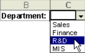
Create a Drop-Down List from a range of cells

In Microsoft Excel, to make data entry easier, or to limit entries to certain items that you define and ensure the correct data is entered, you can create a drop-down list of valid entries that is compiled from cells elsewhere in the workbook. When you create a drop-down list for a cell, it displays an arrow in that cell. To enter information in the cell, click the arrow, and then click the entry that you want.

In this way you don't have to type the data again and again at every occurrence, you simply select it from the drop-down list as picking items from a list. The Data Validation command in the Data Tools group on the Data tab can also be used to achieve this.

• To create a list of valid entries for the drop-down list, type the entries in a single column or row without blank cell as can be seen in this picture below.

• You can sort the data in the order that you want it to appear in the drop-down list.
• If you want to use another worksheet, type the list on that worksheet, and then define a name for the list. (Click Defining Name Reference to read my post on that).
  1. Select the cell where you want the drop-down list.
  2. Click on the Data tab, in the Data Tools group, click Data Validation. The Data Validation dialog box will be displayed.
  3. Click the Settings tab.
  4. In the Allow box, click List.
  5. To specify the location of the list of valid entries, do one of the following:
  • If the list is in the current worksheet, enter a reference to your list in the Source box. For example, enter =Depts or =$C$5:$C$25.
  • If the list is on a different worksheet, enter the name that you defined for your list in the Source box.
  6. Make sure that the In-cell drop-down check box is selected.
  7. Click Ok.