Freeze or Lock Rows and Columns

How Do I Freeze or Lock Rows and Columns in Excel?

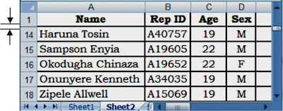
You can view two areas of a worksheet and lock rows or columns in one area by freezing or splitting panes. When you freeze panes, you select specific rows or columns that remain visible and immovable when scrolling in the worksheet. For example, you would freeze panes to keep row and column labels visible as you scroll, as shown in the example below where row 1 is frozen.

When you split panes, you create separate worksheet areas that you can scroll within, while rows or columns in the non-scrolled area remain visible.

Steps to Freeze Panes to lock specific rows or columns

On the worksheet, do one of the following:

1. To lock rows, select the row below where you want the split to appear.
2. To lock columns, select the column to the right of where you want the split to appear.
3. To lock both rows and columns, click the cell below and to the right of where you want the split to appear.

On the View tab, in the Window group, click Freeze Panes, and then click the option that you want.

Split panes to lock rows or columns in separate worksheet areas:

1. To split panes, point to the split box at the top of the vertical scroll bar or at the right end of the horizontal scroll bar.
2. When the mouse pointer changes to a split pointer or , drag the split box down or to the left to the position that you want at the centre of the worksheet.
   
3. To remove the split, double-click any part of the split bar that divides the panes.

This would enable you view or compare different parts of worksheet that are far apart in close range. For instance, you can compare data in column B with data in column AZ at the same time.